Sign-Based Bubble Test (sPWY / sPSY)

radf_sign computes Harvey, Leybourne & Zu (2020)'s sign-based variant of the recursive right-tailed unit root test: instead of applying the (double-)supremum ADF test directly to the series, it is applied to the cumulated sign of its first differences, C_t = sum(sign(diff(y))). Because sign() strips out all magnitude information, C_t's recursive DF statistic is exactly invariant to the pattern of (even time-varying) volatility in the innovations – unlike radf, no wild bootstrap is needed to control size under heteroskedasticity; radf_sign_cv's critical values are pivotal, computed once rather than per dataset.

Usage

radf_sign(data, minw = NULL)

Arguments

data: A univariate or multivariate numeric time series object, a numeric vector or matrix, or a data.frame. A column may have leading and/or trailing NA values (an uneven/unbalanced panel where series enter or exit the sample at different times) – those periods are filled with NA in badf/bsadf and excluded from that series' adf/sadf/ gsadf. Interior NA values (a gap in the middle of a series) are not supported. When any series is padded this way, the panel statistic (bsadf_panel/gsadf_panel) is not available and is returned as NA, with a warning.
minw: A positive integer. The minimum window size (default = \((0.01 + 1.8/\sqrt(T))T\), where T denotes the sample size).

Details

The cost of this invariance is power: the paper finds the sign-based test outperforms the standard PSY test for many time-varying-volatility and bubble specifications, but not all – the standard test can still win for some. The paper's own recommended practical strategy is a bootstrap-based union-of-rejections combining both tests, which is not implemented here (see the package's enhancement notes for the cost/benefit reasoning); this function provides the standalone sign-based test only. sadf is the single-supremum (r1 = 0 fixed) sPWY statistic; gsadf is the double-supremum sPSY statistic.

Note

Needs radf_sign_cv for critical values, not radf_wb_cv or any other bootstrap – the statistic is pivotal (exactly invariant to heteroskedasticity), so its critical values are simulated once, not per dataset.

Carries the radf_obj class and, as of 2026-08-18, its full summary()/datestamp/tidy/autoplot pipeline works – radf_sign_cv() now computes the time-varying badf_cv/bsadf_cv boundary those last two need, not just the three scalar critical values summary() uses. See vignette("naming-and-analysis", package = "exuber").

Level-shift robustness

Harvey, Leybourne, Tatlow & Zu (2025) show this test also retains its standard (no-level-shift) null distribution in the presence of deterministic level shifts, provided the number of shifts grows strictly slower than sqrt(T) – regardless of how large the shifts are. This is a materially weaker requirement than the standard PSY test needs for its own size control, which restricts the number and the magnitude of shifts jointly; in their simulations the standard test is never correctly sized once the number of shifts grows at rate sqrt(T), while this test stays close to nominal size.

Status

References

Harvey, D. I., Leybourne, S. J., & Zu, Y. (2020). Sign-based unit root tests for explosive financial bubbles in the presence of deterministically time-varying volatility. Econometric Theory, 36(1), 122-169.

Harvey, D. I., Leybourne, S. J., Tatlow, D., & Zu, Y. (2025). Unit root tests for explosive financial bubbles in the presence of deterministic level shifts. Oxford Bulletin of Economics and Statistics, 87(5), 879-901. doi:10.1111/obes.12668

Examples

# \donttest{
res <- radf_sign(sim_data, minw = 20)
print(res)
#> 
#> ── radf_sign (minw = 20) ───────────────────────────────────────────────────────
#> 
#>   series      adf    sadf   gsadf
#>     psy1  -0.1516  0.9367   2.021
#>     psy2   2.5578  6.4212  13.985
#>    evans   4.8486  5.7582   6.852
#>      div   1.1346  2.7920   2.950
#>     blan   3.3805  3.3805   3.684
#> 

cv <- radf_sign_cv(n = 100, minw = 20)
summary(res, cv = cv)
#> 
#> ── Summary (minw = 20, lag = 0) ──────────────── Sign-Based MC (nboot = 2000) ──
#> 
#> psy1 :
#> # A tibble: 3 × 5
#>   stat   tstat  `90`  `95`  `99`
#>   <fct>  <dbl> <dbl> <dbl> <dbl>
#> 1 adf   -0.152 0.853  1.27  2.27
#> 2 sadf   0.937 2.17   2.59  3.35
#> 3 gsadf  2.02  2.82   3.33  4.43
#> 
#> psy2 :
#> # A tibble: 3 × 5
#>   stat  tstat  `90`  `95`  `99`
#>   <fct> <dbl> <dbl> <dbl> <dbl>
#> 1 adf    2.56 0.853  1.27  2.27
#> 2 sadf   6.42 2.17   2.59  3.35
#> 3 gsadf 14.0  2.82   3.33  4.43
#> 
#> evans :
#> # A tibble: 3 × 5
#>   stat  tstat  `90`  `95`  `99`
#>   <fct> <dbl> <dbl> <dbl> <dbl>
#> 1 adf    4.85 0.853  1.27  2.27
#> 2 sadf   5.76 2.17   2.59  3.35
#> 3 gsadf  6.85 2.82   3.33  4.43
#> 
#> div :
#> # A tibble: 3 × 5
#>   stat  tstat  `90`  `95`  `99`
#>   <fct> <dbl> <dbl> <dbl> <dbl>
#> 1 adf    1.13 0.853  1.27  2.27
#> 2 sadf   2.79 2.17   2.59  3.35
#> 3 gsadf  2.95 2.82   3.33  4.43
#> 
#> blan :
#> # A tibble: 3 × 5
#>   stat  tstat  `90`  `95`  `99`
#>   <fct> <dbl> <dbl> <dbl> <dbl>
#> 1 adf    3.38 0.853  1.27  2.27
#> 2 sadf   3.38 2.17   2.59  3.35
#> 3 gsadf  3.68 2.82   3.33  4.43
#> 
tidy(res, cv = cv)
#> # A tibble: 5 × 4
#>   id       adf  sadf gsadf
#>   <fct>  <dbl> <dbl> <dbl>
#> 1 psy1  -0.152 0.937  2.02
#> 2 psy2   2.56  6.42  14.0 
#> 3 evans  4.85  5.76   6.85
#> 4 div    1.13  2.79   2.95
#> 5 blan   3.38  3.38   3.68
datestamp(res, cv = cv)
#> 
#> ── Datestamp (min_duration = 0) ─────────────────────────────── Sign-Based MC ──
#> 
#> psy2 :
#>   Start Peak End Duration   Signal Ongoing
#> 1    21   40 100       80 positive    TRUE
#> 
#> evans :
#>   Start Peak End Duration   Signal Ongoing
#> 1    21   84 100       80 positive    TRUE
#> 
#> blan :
#>   Start Peak End Duration   Signal Ongoing
#> 1    31   43  52       21 negative   FALSE
#> 2    53   58  73       20 positive   FALSE
#> 3    77  100 100       24 positive    TRUE
#> 
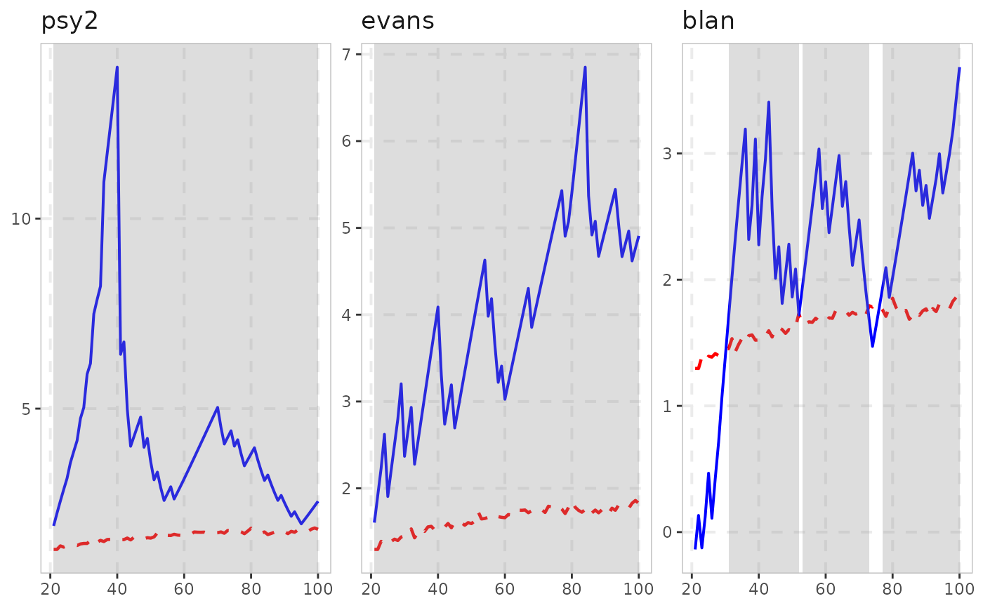
autoplot(res, cv = cv)

# }