The following function generates a time series which switches from a martingale to a mildly explosive process and then back to a martingale.
sim_psy1(
  n,
  te = 0.4 * n,
  tf = 0.15 * n + te,
  c = 1,
  alpha = 0.6,
  sigma = 6.79,
  seed = NULL
)
Arguments
- n
A positive integer specifying the length of the simulated output series.
- te
A scalar in (0, tf) specifying the observation in which the bubble originates.
- tf
A scalar in (te, n) specifying the observation in which the bubble collapses.
- c
A positive scalar determining the autoregressive coefficient in the explosive regime.
- alpha
A positive scalar in (0, 1) determining the value of the expansion rate in the autoregressive coefficient.
- sigma
A positive scalar indicating the standard deviation of the innovations.
- seed
An object specifying if and how the random number generator (rng) should be initialized. Either NULL or an integer will be used in a call to
set.seedbefore simulation. If set, the value is saved as "seed" attribute of the returned value. The default, NULL, will not change rng state, and return .Random.seed as the "seed" attribute. Results are different between the parallel and non-parallel option, even if they have the same seed.
Value
A numeric vector of length n.
Details
The data generating process is described by the following equation: $$X_t = X_{t-1}1\{t < \tau_e\}+ \delta_T X_{t-1}1\{\tau_e \leq t\leq \tau_f\} + \left(\sum_{k=\tau_f+1}^t \epsilon_k + X_{\tau_f}\right) 1\{t > \tau_f\} + \epsilon_t 1\{t \leq \tau_f\} $$
where the autoregressive coefficient \(\delta_T\) is given by:
$$\delta_T = 1 + cT^{-a}$$
with \(c>0\), \(\alpha \in (0,1)\), \(\epsilon \sim iid(0, \sigma^2)\) and \(X_{\tau_f} = X_{\tau_e} + X'\) with \(X' = O_p(1)\), \(\tau_e = [T r_e]\) dates the origination of the bubble, and \(\tau_f = [T r_f]\) dates the collapse of the bubble. During the pre- and post- bubble periods, \([1, \tau_e)\), \(X_t\) is a pure random walk process. During the bubble expansion period \(\tau_e, \tau_f]\) becomes a mildly explosive process with expansion rate given by the autoregressive coefficient \(\delta_T\); and, finally during the post-bubble period, \((\tau_f, \tau]\) \(X_t\) reverts to a martingale.
For further details see Phillips et al. (2015) p. 1054.
References
Phillips, P. C. B., Shi, S., & Yu, J. (2015). Testing for Multiple Bubbles: Historical Episodes of Exuberance and Collapse in the S&P 500. International Economic Review, 5 6(4), 1043-1078.
Examples
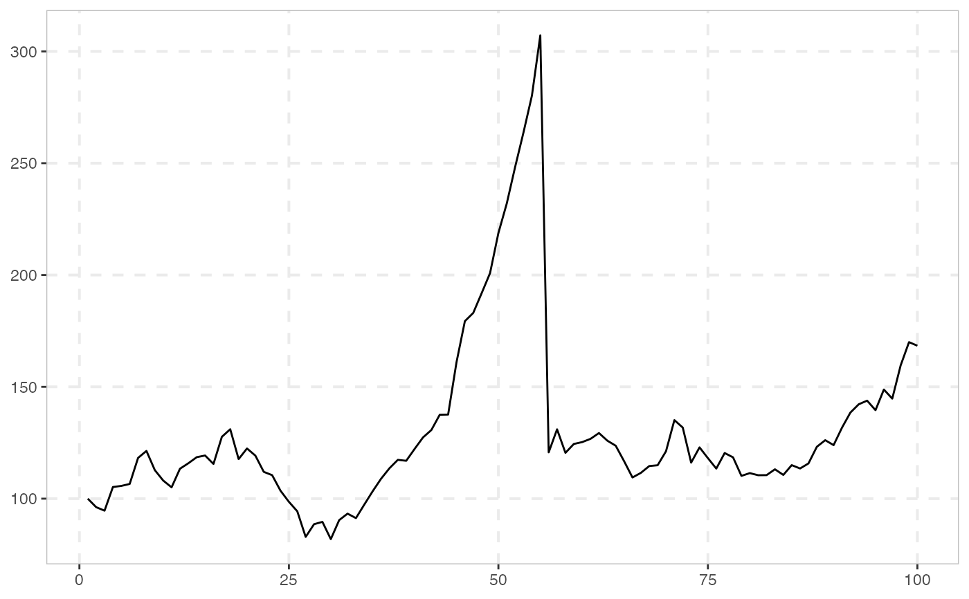
# 100 periods with bubble origination date 40 and termination date 55
sim_psy1(n = 100, seed = 123) %>%
autoplot()
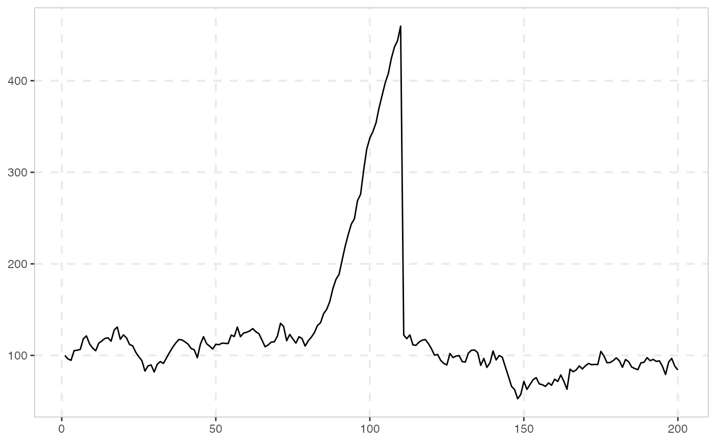
 # 200 periods with bubble origination date 80 and termination date 110
sim_psy1(n = 200, seed = 123) %>%
autoplot()
# 200 periods with bubble origination date 80 and termination date 110
sim_psy1(n = 200, seed = 123) %>%
autoplot()
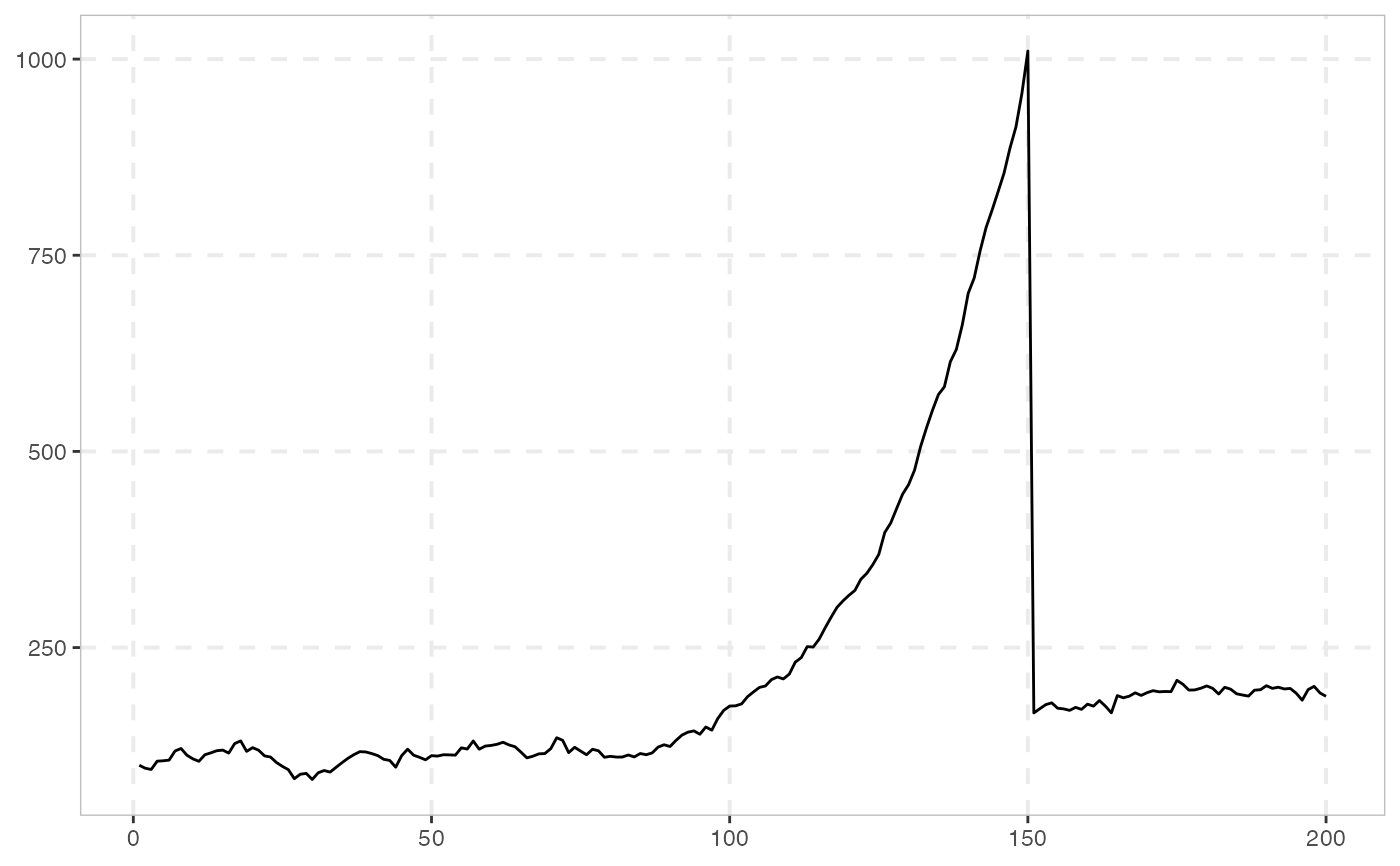
 # 200 periods with bubble origination date 100 and termination date 150
sim_psy1(n = 200, te = 100, tf = 150, seed = 123) %>%
autoplot()
# 200 periods with bubble origination date 100 and termination date 150
sim_psy1(n = 200, te = 100, tf = 150, seed = 123) %>%
autoplot()