radf_wb_cv performs the Harvey et al. (2016) wild bootstrap re-sampling
scheme, which is asymptotically robust to non-stationary volatility, to
generate critical values for the recursive unit root tests. radf_wb_distr
computes the distribution.
radf_wb_cv(data, minw = NULL, nboot = 500L, dist_rad = FALSE, seed = NULL)

radf_wb_distr(data, minw = NULL, nboot = 500L, dist_rad = FALSE, seed = NULL)
Arguments
- data
A univariate or multivariate numeric time series object, a numeric vector or matrix, or a data.frame. The object should not have any NA values.
- minw
A positive integer. The minimum window size (default = \((0.01 + 1.8/\sqrt(T))T\), where T denotes the sample size).
- nboot
A positive integer. Number of bootstraps (default = 500L).
- dist_rad
Logical. If TRUE then the Rademacher distribution will be used.
- seed
An object specifying if and how the random number generator (rng) should be initialized. Either NULL or an integer will be used in a call to
set.seedbefore simulation. If set, the value is saved as "seed" attribute of the returned value. The default, NULL, will not change rng state, and return .Random.seed as the "seed" attribute. Results are different between the parallel and non-parallel option, even if they have the same seed.
Value
For radf_wb_cv a list that contains the critical values for the ADF,
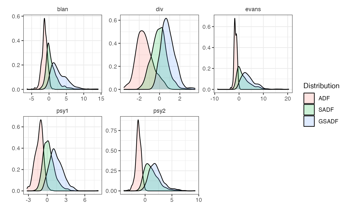
BADF, BSADF and GSADF tests. For radf_wb_distr a list that
contains the ADF, SADF and GSADF distributions.
Details
This approach involves applying a wild bootstrap re-sampling scheme to construct the bootstrap analogue of the Phillips et al. (2015) test which is asymptotically robust to non-stationary volatility.
References
Harvey, D. I., Leybourne, S. J., Sollis, R., & Taylor, A. M. R. (2016). Tests for explosive financial bubbles in the presence of non-stationary volatility. Journal of Empirical Finance, 38(Part B), 548-574.
Phillips, P. C. B., Shi, S., & Yu, J. (2015). Testing for Multiple Bubbles: Historical Episodes of Exuberance and Collapse in the S&P 500. International Economic Review, 56(4), 1043-1078.
See also
radf_mc_cv for Monte Carlo critical values and
radf_sb_cv for sieve bootstrap critical values.
Examples
# \donttest{
# Default minimum window
wb <- radf_wb_cv(sim_data)

tidy(wb)
#> # A tibble: 15 × 5
#>    id    sig       adf  sadf gsadf
#>    <fct> <fct>   <dbl> <dbl> <dbl>
#>  1 psy1  90    -0.572   1.53  2.87
#>  2 psy2  90    -0.625   3.29  4.09
#>  3 evans 90    -0.525   6.74  8.82
#>  4 div   90    -0.418   1.03  1.76
#>  5 blan  90    -0.199   3.11  6.46
#>  6 psy1  95    -0.411   1.96  3.44
#>  7 psy2  95    -0.511   4.01  4.72
#>  8 evans 95    -0.312   9.25 10.5
#>  9 div   95    -0.0990  1.34  2.11
#> 10 blan  95     0.0461  4.14  7.86
#> 11 psy1  99     0.104   2.71  4.70
#> 12 psy2  99    -0.266   5.43  6.80
#> 13 evans 99    -0.0136 14.0  15.9
#> 14 div   99     0.425   1.93  2.64
#> 15 blan  99     0.402   7.67 12.1

# Change the minimum window and the number of bootstraps
wb2 <- radf_wb_cv(sim_data, nboot = 600, minw = 20)

tidy(wb2)
#> # A tibble: 15 × 5
#>    id    sig        adf   sadf gsadf
#>    <fct> <fct>    <dbl>  <dbl> <dbl>
#>  1 psy1  90    -0.577    1.50   2.72
#>  2 psy2  90    -0.623    3.16   4.04
#>  3 evans 90    -0.625    5.06   7.76
#>  4 div   90    -0.472    0.988  1.63
#>  5 blan  90    -0.354    2.93   5.97
#>  6 psy1  95    -0.392    1.85   3.16
#>  7 psy2  95    -0.527    3.86   4.87
#>  8 evans 95    -0.442    7.28   9.51
#>  9 div   95    -0.0674   1.26   2.03
#> 10 blan  95    -0.101    4.12   7.78
#> 11 psy1  99     0.00929  2.78   4.39
#> 12 psy2  99    -0.294    5.12   6.84
#> 13 evans 99    -0.0690  11.8   12.7
#> 14 div   99     0.670    1.81   2.80
#> 15 blan  99     0.427    5.92  10.4

# Simulate distribution
wdist <- radf_wb_distr(sim_data)

autoplot(wdist)

# }
# }