
Why another test
radf(), the classic PSY GSADF test, assumes that the
innovation variance is constant. Real financial series usually do not
have constant volatility. Harvey, Leybourne, Sollis & Taylor (2016)
show that when volatility changes over time, the standard critical
values of radf() no longer control the size of the test.
radf_wb_cv() addresses this in exuber with a wild
bootstrap.
radf_tt() implements a different fix that needs no
bootstrap, from Kurozumi, Skrobotov & Tsarev (2024, Journal of
Financial Econometrics). Instead of resampling, it time-deforms the
series using a nonparametric estimate of its variance profile, so that
under the null the deformed series behaves like a random walk with
constant volatility. The null distribution of the resulting statistic is
then the same pivotal distribution as under homoskedasticity. Ordinary
asymptotic critical values therefore apply, with no bootstrap and no
resimulation for each dataset.
Basic usage
radf_tt() targets non-stationary volatility, meaning a
permanent shift or trend in the unconditional innovation variance, which
is the setting of the simulations in Kurozumi, Skrobotov & Tsarev.
It does not target stationary conditional heteroskedasticity such as
GARCH. In that case the variance profile is asymptotically flat, the
time deformation is close to the identity, and plain radf()
already has the correct size. sim_vol_break() generates
innovations with a permanent volatility shift, and the e
argument of sim_psy1() passes them into the PSY bubble
process. Here the innovation standard deviation triples half-way through
the sample:
y <- sim_psy1(n = 200, seed = 1, e = sim_vol_break(199))
res <- radf_tt(y)
res
#>
#> ── radf_tt (minw = 27, kernel = uniform) ───────────────────────────────────────
#>
#>    series      adf   sadf  gsadf
#>   series1  -0.9972  3.275  4.165
radf_tt_cv() returns the matching pivotal asymptotic
critical values. The null distribution does not depend on the volatility
path, so one call with a large n approximates the whole
family of cases. radf_wb_cv(), in contrast, runs a separate
bootstrap for each dataset:
cv <- radf_tt_cv(n = 300, minw = 30, nrep = 1000, seed = 1)
cv$gsadf_cv
#>      90%      95%      99%
#> 3.248911 3.584415 4.246916
What is estimated
radf_tt() works in three steps.
- It estimates the time-varying AR(1) coefficient with a local kernel
regression. From the truncated residuals it builds a monotone variance
profile
eta_hat(s), withsin[0, 1]. - It inverts the profile and uses the inverse to resample and time-deform the series.
- It computes a recursive sup-ADF statistic (GLS-demeaned, with no
intercept) on the deformed series. This belongs to the same family of
statistics as
radf(), but it needs no fitted intercept, which matches the derivation in the paper.
You can adjust kernel ("uniform", the
choice of the paper, or "gaussian") and h, the
bandwidth. The default for h is a fixed plug-in value and
not the full cross-validation search of the paper.
Dating and plotting a detected bubble
radf_tt() returns the same radf_obj class
as radf(). radf_tt_cv() also computes the full
time-varying boundary that dating and plotting need, and not only the
summary-level critical values. The usual pipeline therefore works
unchanged:
res <- radf_tt(y, minw = 20)
cv <- radf_tt_cv(n = 200, minw = 20)

datestamp(res, cv = cv)
#>
#> ── Datestamp (min_duration = 0) ───────────────────────── Time-Transformed MC ──
#>
#> series1 :
#>   Start Peak End Duration   Signal Ongoing
#> 1    21   38  89       68 negative   FALSE
#> 2   148  148 150        2 positive   FALSE
autoplot(res, cv = cv)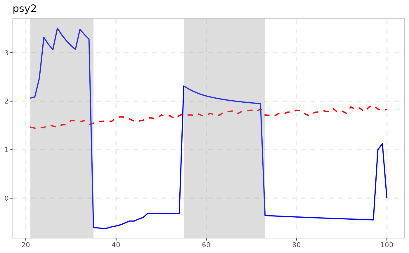
vignette("naming-and-analysis") explains which other
exuber functions work with this pipeline and which do not.