Time-Transformed Test for Explosive Bubbles under Non-stationary Volatility

radf_tt computes the STADF/GSTADF test statistics of Kurozumi, Skrobotov & Tsarev, a heteroskedasticity-robust alternative to radf that requires no bootstrap: the series is time-deformed using a nonparametric estimate of its variance profile, after which the usual (asymptotic, homoskedastic) recursive sup-ADF critical values apply.

Usage

radf_tt(data, minw = NULL, kernel = c("uniform", "gaussian"), h = NULL)

Arguments

data

A univariate or multivariate numeric time series object, a numeric vector or matrix, or a data.frame. A column may have leading and/or trailing NA values (an uneven/unbalanced panel where series enter or exit the sample at different times) – those periods are filled with NA in badf/bsadf and excluded from that series' adf/sadf/ gsadf. Interior NA values (a gap in the middle of a series) are not supported. When any series is padded this way, the panel statistic (bsadf_panel/gsadf_panel) is not available and is returned as NA, with a warning.

minw

A positive integer. The minimum window size (default = \((0.01 + 1.8/\sqrt(T))T\), where T denotes the sample size).

kernel

Kernel used in the local variance-profile regression, "uniform" (default, as in the paper's simulations) or "gaussian".

h

Bandwidth for the variance-profile kernel regression. Default T^(-2/5), the midpoint (on the log scale) of the paper's cross-validation search range \([T^{-0.5}, T^{-0.3}]\).

Details

For critical values, use radf_tt_cv as the primary recommendation: it is pivotal (asymptotically free of the volatility process), so it does not need to be recomputed per dataset, unlike a bootstrap. radf_wb_cv (Harvey, Leybourne, Sollis & Taylor's wild bootstrap) is a bootstrap-based alternative, worth considering if non-pivotality/finite-sample bootstrap robustness is a specific concern.

Note

Carries the radf_obj class and, as of 2026-08-18, its full summary()/datestamp/tidy/autoplot pipeline works – radf_tt_cv() now computes the time-varying badf_cv/bsadf_cv boundary those last two need, not just the three scalar critical values summary() uses. See vignette("naming-and-analysis", package = "exuber").

References

Kurozumi, E., Skrobotov, A., & Tsarev, A. (2024). Time-Transformed Test for Bubbles under Non-stationary Volatility. Journal of Financial Econometrics. doi:10.1093/jjfinec/nbae026

See also

radf_tt_cv for the (pivotal, bootstrap-free) asymptotic critical values, and radf_wb_cv for the bootstrap-based alternative (Harvey, Leybourne, Sollis & Taylor).

Examples

# \donttest{
res <- radf_tt(sim_data, minw = 20)
print(res)
#> 
#> ── radf_tt (minw = 20, kernel = uniform) ───────────────────────────────────────
#> 
#>   series      adf    sadf  gsadf
#>     psy1  -1.0366  1.2750  2.204
#>     psy2  -0.8600  2.5960  3.505
#>    evans  -1.3349  1.6556  1.883
#>      div   0.7217  2.3440  2.344
#>     blan  -1.3363  0.4998  1.541
#> 

cv <- radf_tt_cv(n = 100, minw = 20)
summary(res, cv = cv)
#> 
#> ── Summary (minw = 20, lag = 0) ────────── Time-Transformed MC (nboot = 2000) ──
#> 
#> psy1 :
#> # A tibble: 3 × 5
#>   stat  tstat  `90`  `95`  `99`
#>   <fct> <dbl> <dbl> <dbl> <dbl>
#> 1 adf   -1.04 0.978  1.36  2.02
#> 2 sadf   1.27 2.21   2.55  3.25
#> 3 gsadf  2.20 2.84   3.22  3.90
#> 
#> psy2 :
#> # A tibble: 3 × 5
#>   stat   tstat  `90`  `95`  `99`
#>   <fct>  <dbl> <dbl> <dbl> <dbl>
#> 1 adf   -0.860 0.978  1.36  2.02
#> 2 sadf   2.60  2.21   2.55  3.25
#> 3 gsadf  3.50  2.84   3.22  3.90
#> 
#> evans :
#> # A tibble: 3 × 5
#>   stat  tstat  `90`  `95`  `99`
#>   <fct> <dbl> <dbl> <dbl> <dbl>
#> 1 adf   -1.33 0.978  1.36  2.02
#> 2 sadf   1.66 2.21   2.55  3.25
#> 3 gsadf  1.88 2.84   3.22  3.90
#> 
#> div :
#> # A tibble: 3 × 5
#>   stat  tstat  `90`  `95`  `99`
#>   <fct> <dbl> <dbl> <dbl> <dbl>
#> 1 adf   0.722 0.978  1.36  2.02
#> 2 sadf  2.34  2.21   2.55  3.25
#> 3 gsadf 2.34  2.84   3.22  3.90
#> 
#> blan :
#> # A tibble: 3 × 5
#>   stat   tstat  `90`  `95`  `99`
#>   <fct>  <dbl> <dbl> <dbl> <dbl>
#> 1 adf   -1.34  0.978  1.36  2.02
#> 2 sadf   0.500 2.21   2.55  3.25
#> 3 gsadf  1.54  2.84   3.22  3.90
#> 
tidy(res, cv = cv)
#> # A tibble: 5 × 4
#>   id       adf  sadf gsadf
#>   <fct>  <dbl> <dbl> <dbl>
#> 1 psy1  -1.04  1.27   2.20
#> 2 psy2  -0.860 2.60   3.50
#> 3 evans -1.33  1.66   1.88
#> 4 div    0.722 2.34   2.34
#> 5 blan  -1.34  0.500  1.54
datestamp(res, cv = cv)
#> 
#> ── Datestamp (min_duration = 0) ───────────────────────── Time-Transformed MC ──
#> 
#> psy2 :
#>   Start Peak End Duration   Signal Ongoing
#> 1    21   27  35       14 positive   FALSE
#> 2    55   55  73       18 positive   FALSE
#> 
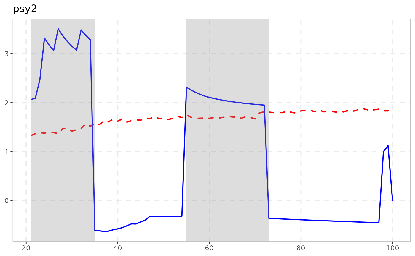
autoplot(res, cv = cv)

# }