Kernel-Purged Heteroskedasticity-Robust PSY Test

radf_kp implements the heteroskedasticity-robust PSY test of Harvey, Leybourne, Taylor & Zu (2024), which needs no bootstrap. It "purges" unconditional heteroskedasticity by dividing each first difference of the series by a kernel spot-volatility estimate (eq. 4-5) and cumulating the result. It then runs the ordinary radf, with an intercept, on the purged series.

Usage

radf_kp(data, minw = NULL, kernel = c("gaussian", "uniform"), h = NULL)

Arguments

data

A univariate or multivariate numeric time series object, a numeric vector or matrix, or a data.frame. A column may have leading or trailing NA values, which describes an unbalanced panel in which series enter or exit the sample at different times. Those periods are filled with NA in badf and bsadf and excluded from the adf, sadf and gsadf of that series. Interior NA values (a gap in the middle of a series) are not supported. When any series is padded in this way, the panel statistics (bsadf_panel and gsadf_panel) are not available, and the function returns NA for them with a warning.

minw

A positive integer. The minimum window size (default = \((0.01 + 1.8/\sqrt{T})T\), where T denotes the sample size).

kernel

Kernel for the spot-volatility estimator, "gaussian" (default, as in the paper) or "uniform".

h

Bandwidth for the spot-volatility estimator. The default is 0.1 * T^(-0.25), the setting of the paper (Table I, Section 6).

Value

A radf_obj with the same structure as the output of radf, computed on the volatility-purged series, so radf_mc_cv, tidy() and the other methods apply directly.

Details

The paper proves (Theorem 1 and Remark 3.2) that the null limiting distribution of the purged statistic is identical to the standard homoskedastic GSADF null. radf_mc_cv, the existing and already fast Monte Carlo critical values of exuber, therefore apply directly to the result. Unlike radf_wb_cv and radf_sbz_cv, no new bootstrap or simulation code is needed.

Only the with-intercept variant (\(PSY_\sigma\) in the paper) is implemented. The paper also proposes a variant without an intercept and a union-of-rejections test that combines both. They are not implemented here (see the package's enhancement notes for the cost and benefit considerations).

Note

The function returns the unmodified output of radf, so the full summary(), datestamp, tidy and autoplot pipeline works exactly as it does for plain radf() (see vignette("naming-and-analysis", package = "exuber")).

Status

References

Harvey, D. I., Leybourne, S. J., Taylor, A. M. R., & Zu, Y. (2024). A new heteroskedasticity-robust test for explosive bubbles. Journal of Time Series Analysis. doi:10.1111/jtsa.12784

See also

radf_mc_cv for the critical values of this test, which are unmodified, radf_wb_cv for a bootstrap-based alternative, and radf_tt for another alternative that needs no bootstrap.

Other volatility-robust tests: cusum_test(), radf_sbz(), radf_sbz_union(), radf_sign(), radf_sign_dm(), radf_tt(), ssu_test()

Examples

# \donttest{
# Volatility triples half-way through the sample. This is the case of
# non-stationary volatility that this test is built for, and plain radf()
# over-rejects here
y <- sim_psy1(n = 200, seed = 1, e = sim_vol_break(199))
res <- radf_kp(y, minw = 20)
print(res)
#> 
#> ── radf (minw = 20, lag = 0) ───────────────────────────────────────────────────
#> 
#>        id     adf   sadf  gsadf
#>   series1  -1.715  1.503  2.633
#> 
#>   gsadf_panel
#>         2.633
#> 

# radf_mc_cv() applies unmodified (see Details)
cv <- radf_mc_cv(n = attr(res, "n"), minw = 20)
summary(res, cv = cv)
#> 
#> ── Summary (minw = 20, lag = 0) ────────────────── Monte Carlo (nboot = 1000) ──
#> 
#> series1 :
#> # A tibble: 3 × 5
#>   stat  tstat   `90`    `95`  `99`
#>   <fct> <dbl>  <dbl>   <dbl> <dbl>
#> 1 adf   -1.72 -0.328 0.00172 0.572
#> 2 sadf   1.50  1.19  1.48    1.97 
#> 3 gsadf  2.63  1.99  2.27    2.87 
#> 
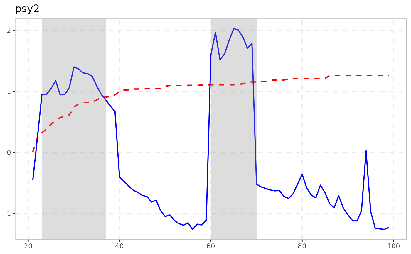
autoplot(res, cv = cv)

# }