WLS/Kernel-Volatility Bubble Statistic (SBZ)

radf_sbz computes the WLS (kernel-volatility-weighted) recursive sup-ADF statistic of Harvey, Leybourne & Zu (2019) – supBZ in their own notation – via wls_dfstat_grid() (internal), returning the same shape radf itself does (adf/sadf/gsadf scalars plus the full badf/bsadf recursive paths), so it carries the radf_obj class and the full summary()/ datestamp/tidy/autoplot pipeline works, paired with radf_sbz_cv.

Usage

radf_sbz(data, minw = NULL, kernel = c("gaussian", "uniform"), h = NULL)

Arguments

data: A univariate or multivariate numeric time series object, a numeric vector or matrix, or a data.frame. A column may have leading and/or trailing NA values (an uneven/unbalanced panel where series enter or exit the sample at different times) – those periods are filled with NA in badf/bsadf and excluded from that series' adf/sadf/ gsadf. Interior NA values (a gap in the middle of a series) are not supported. When any series is padded this way, the panel statistic (bsadf_panel/gsadf_panel) is not available and is returned as NA, with a warning.
minw: A positive integer. The minimum window size (default = \((0.01 + 1.8/\sqrt(T))T\), where T denotes the sample size).
kernel: Kernel for the spot-volatility estimator (eq. 6 of Harvey, Leybourne & Zu 2019), "gaussian" (default, as in the paper) or "uniform".
h: Bandwidth for the spot-volatility estimator. Default: leave-one-out cross-validation over the paper's own search range.

Value

An object of class radf_sbz_obj/radf_obj: a list with adf, sadf, gsadf (one value per series) and badf, bsadf (matrices, one column per series).

Details

Unlike the bundled radf_sbz_union (which combines this with the classic supDF statistic into a bootstrap-calibrated union test), supBZ alone needs no bootstrap to be defined – only to be tested – so it splits into a statistic and a critical-value function the way most of exuber does.

Note

Needs radf_sbz_cv for critical values, not radf_wb_cv or radf_mc_cv – supBZ's own null distribution depends on the WLS weighting, so it needs its own (data-dependent, wild-bootstrap) critical value function, same reasoning as radf()/radf_wb_cv.

Status

References

Harvey, D. I., Leybourne, S. J., & Zu, Y. (2019). Testing explosive bubbles with time-varying volatility. Econometric Reviews, 38(10), 1131-1151.

Examples

# \donttest{
res <- radf_sbz(sim_data, minw = 20)
print(res)
#> 
#> ── radf (minw = 20, lag = 0) ───────────────────────────────────────────────────
#> 
#>      id      adf     sadf  gsadf
#>    psy1  -1.2166   0.2802  1.047
#>    psy2  -1.0665   1.5349  1.563
#>   evans  -2.9534  -1.0012  1.705
#>     div   0.6601   2.2607  2.261
#>    blan  -4.1432   1.4008  2.381
#> 
#> [1] gsadf_panel
#> <0 rows> (or 0-length row.names)
#> 

cv <- radf_sbz_cv(sim_data, minw = 20, nboot = 200)
summary(res, cv = cv)
#> 
#> ── Summary (minw = 20, lag = 0) ────────── Wild Bootstrap (SBZ) (nboot = 200) ──
#> 
#> psy1 :
#> # A tibble: 3 × 5
#>   stat   tstat  `90`  `95`  `99`
#>   <fct>  <dbl> <dbl> <dbl> <dbl>
#> 1 adf   -1.22  0.623 0.826  1.18
#> 2 sadf   0.280 1.62  1.97   2.54
#> 3 gsadf  1.05  1.96  2.84   3.87
#> 
#> psy2 :
#> # A tibble: 3 × 5
#>   stat  tstat  `90`  `95`  `99`
#>   <fct> <dbl> <dbl> <dbl> <dbl>
#> 1 adf   -1.07 0.476 0.615 0.833
#> 2 sadf   1.53 2.13  2.65  4.39 
#> 3 gsadf  1.56 2.52  3.11  5.58 
#> 
#> evans :
#> # A tibble: 3 × 5
#>   stat  tstat  `90`  `95`  `99`
#>   <fct> <dbl> <dbl> <dbl> <dbl>
#> 1 adf   -2.95 0.589 0.806 0.993
#> 2 sadf  -1.00 4.04  5.44  7.43 
#> 3 gsadf  1.70 4.65  5.75  8.23 
#> 
#> div :
#> # A tibble: 3 × 5
#>   stat  tstat  `90`  `95`  `99`
#>   <fct> <dbl> <dbl> <dbl> <dbl>
#> 1 adf   0.660 0.922  1.24  1.94
#> 2 sadf  2.26  2.07   2.37  3.13
#> 3 gsadf 2.26  2.39   2.75  3.31
#> 
#> blan :
#> # A tibble: 3 × 5
#>   stat  tstat  `90`  `95`  `99`
#>   <fct> <dbl> <dbl> <dbl> <dbl>
#> 1 adf   -4.14 0.609  1.09  1.39
#> 2 sadf   1.40 2.44   3.51  7.38
#> 3 gsadf  2.38 3.28   4.43  7.57
#> 
tidy(res, cv = cv)
#> # A tibble: 5 × 4
#>   id       adf   sadf gsadf
#>   <fct>  <dbl>  <dbl> <dbl>
#> 1 psy1  -1.22   0.280  1.05
#> 2 psy2  -1.07   1.53   1.56
#> 3 evans -2.95  -1.00   1.70
#> 4 div    0.660  2.26   2.26
#> 5 blan  -4.14   1.40   2.38

# datestamp()/autoplot() need at least one rejection; supBZ's
# kernel-volatility weighting trades away enough power that none of
# sim_data's five series clear it, so use a series built to reject:
set.seed(7)
n <- 120; te <- 70
y <- cumsum(rnorm(n))
y[(te + 1):n] <- y[te] * 1.15 ^ seq_len(n - te)
res2 <- radf_sbz(y, minw = 20)
cv2 <- radf_sbz_cv(y, minw = 20, nboot = 100, seed = 1)
datestamp(res2, cv = cv2)
#> 
#> ── Datestamp (min_duration = 0) ──────────────────────── Wild Bootstrap (SBZ) ──
#> 
#> series1 :
#>   Start Peak End Duration   Signal Ongoing
#> 1    27   28  29        2 positive   FALSE
#> 2    64  120 120       57 positive    TRUE
#> 
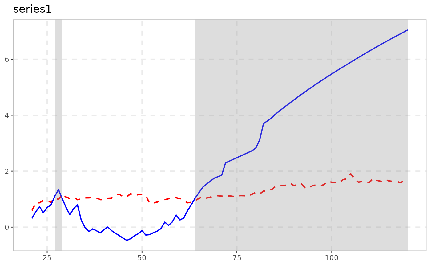
autoplot(res2, cv = cv2)

# }