Monte Carlo critical values for the time-transformed test (STADF/GSTADF)

This is the dedicated critical-value function for radf_tt. It simulates the asymptotic null distribution of the GLS-demeaned recursive sup-ADF statistic used by radf_tt. Per Theorem 1 of Kurozumi, Skrobotov & Tsarev, this distribution is free of the volatility process (pivotal), so – unlike radf_wb_cv – it does not need to be recomputed per dataset: a large n with default nrep well approximates the T -> Inf limit used in the paper.

Usage

radf_tt_cv(n, minw = NULL, nrep = 2000L, seed = NULL)

Arguments

n: A positive integer. The sample size.
minw: A positive integer. The minimum window size (default = \((0.01 + 1.8/\sqrt(T))T\), where T denotes the sample size).
nrep: A positive integer. The number of Monte Carlo simulations.
seed: An object specifying if and how the random number generator (rng) should be initialized. Either NULL or an integer will be used in a call to set.seed before simulation. If set, the value is saved as "seed" attribute of the returned value. The default, NULL, will not change rng state, and return .Random.seed as the "seed" attribute. Results are reproducible across the parallel and non-parallel option when the same seed is used.

Details

The sadf_cv column (STADF, i.e. r1 = 0 fixed) can be checked against Whitehouse (2019)'s published asymptotic values, quoted in Kurozumi, Skrobotov & Tsarev's footnote 4: for minw/n = 0.1, (10\ 5\ STADF, not GSTADF (gsadf_cv) – the paper's own GSTADF critical values are not given as literal numbers in the text, only as "easily computed from" the authors' R code.

Note

As of 2026-08-18, also computes badf_cv/bsadf_cv (a time-varying boundary, one row per recursion point), so datestamp/autoplot now work on radf_tt results, not just summary()/tidy. Unlike radf_mc_cv's own bsadf_cv (a cummax()-across- replicates shortcut around the base C++ engine's output shape), gls_dfstat_grid()'s (internal) bsadf is already the genuine sup-over-all-window-starts statistic at each point, so no such shortcut is needed here – just the per-time-point quantile across replicates. Validated: badf_cv's last row is bit-identical to adf_cv (a hard identity, since adf is literally badf's last point, per replicate); empirical false-alarm rate under H0 is conservative relative to nominal (3.3\ nrep=2000); and detection power on a synthetic bubble matches the established radf()/radf_mc_cv() pipeline almost exactly (18\ radf_sign_dm_cv() have the same gap, not yet addressed the same way – see vignette("naming-and-analysis").

References

Kurozumi, E., Skrobotov, A., & Tsarev, A. (2024). Time-Transformed Test for Bubbles under Non-stationary Volatility. Journal of Financial Econometrics. doi:10.1093/jjfinec/nbae026

Examples

# \donttest{
cv <- radf_tt_cv(n = 100, minw = 20)
tidy(cv)
#> # A tibble: 3 × 4
#>   sig     adf  sadf gsadf
#>   <fct> <dbl> <dbl> <dbl>
#> 1 90    0.873  2.12  2.75
#> 2 95    1.31   2.50  3.17
#> 3 99    2.07   3.10  4.01

res <- radf_tt(sim_data, minw = 20)
datestamp(res, cv = cv)
#> 
#> ── Datestamp (min_duration = 0) ───────────────────────── Time-Transformed MC ──
#> 
#> psy2 :
#>   Start Peak End Duration   Signal Ongoing
#> 1    21   27  35       14 positive   FALSE
#> 2    55   55  73       18 positive   FALSE
#> 
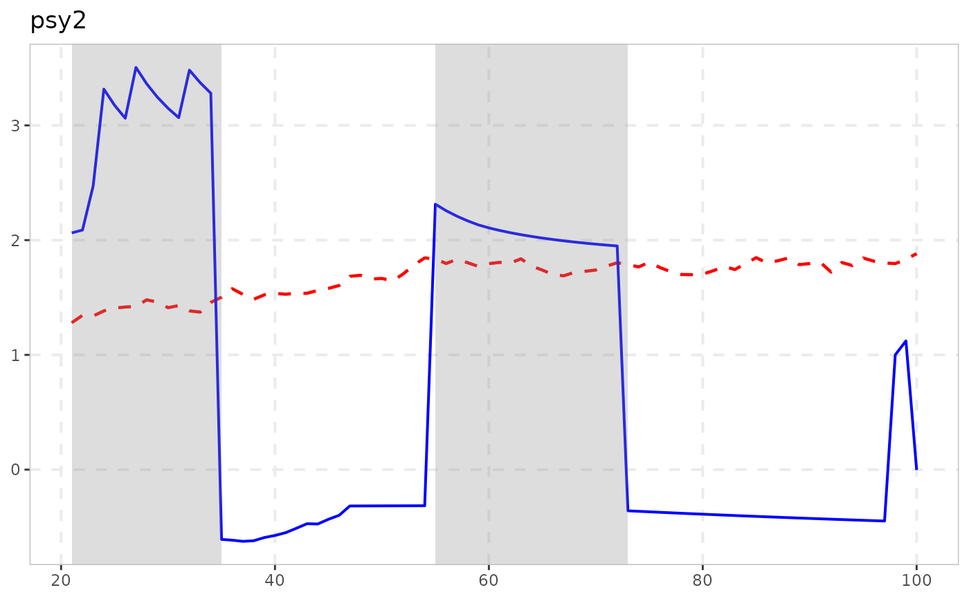
autoplot(res, cv = cv)

# }