
Sequential LBI Monitoring for an Unknown Bubble Start Date (Breitung & Diegel 2025)
Source:R/lbi_test.R
monitor_lbi.Rdmonitor_lbi implements the sequential, constant-boundary extension of the
locally best invariant statistic of lbi_test. It monitors a series
in real time when the start date of the bubble is unknown. After a training
window [1, T*] that is assumed free of exuberance, it compares the
(optionally exponentially weighted) partial sum of the post-training first
differences with a constant boundary and flags the first monitoring date at
which the boundary is breached.
Arguments
- data
A univariate or multivariate numeric time series object, a numeric vector or matrix, or a data.frame. A column may have leading or trailing
NAvalues, which describes an unbalanced panel in which series enter or exit the sample at different times. Those periods are filled withNAinbadfandbsadfand excluded from theadf,sadfandgsadfof that series. InteriorNAvalues (a gap in the middle of a series) are not supported. When any series is padded in this way, the panel statistics (bsadf_panelandgsadf_panel) are not available, and the function returnsNAfor them with a warning.- r_star
The end of the training window: a fraction in
(0, 1)of the sample (default0.5), or an integer number of observations if>= 1.- c_bar
Exponential up-weighting parameter for later monitoring observations, which are more likely to be bubble-like (their eq. 12),
>= 0. The default0is the flat-weight "mCUSUM" variant, which is appropriate when a bubble is equally likely to start at any point in the monitoring window. For a moderate gain in power when a bubble that starts partway through the window is more plausible, the paper suggests2. The critical values (sig_lvl) are the same for everyc_bar.- sig_lvl
Significance level on the 0 to 100 scale used throughout the package, one of
90,95,97.5,99or99.5. Table 1 of Breitung & Diegel tabulates only these.
Value
An object of class monitor_lbi_obj: a list with the statistic path
in the monitoring region (stat), the constant boundary, the length
of the training window T_star, and alarm and alarm_date (the
first breach, NA if there is none).
Details
Their eq. 15 shows that this partial sum, normalized by the fixed length of the
monitoring horizon, converges to a standard Brownian motion on [0, 1]
under the null. The normalization is not sqrt(t), which differs from the
Chu-Stinchcombe-White-style boundary of monitor_cusum. A single
constant boundary therefore controls size uniformly across the whole monitoring
window. The paper shows that this constant-boundary detector ("mCUSUM" at
c_bar = 0, "wCUSUM" at c_bar > 0) is more powerful than the
classical CUSUM test with a time-varying boundary, to which it is compared.
Note
The critical value is the published constant boundary in Table 1 of Breitung & Diegel (2025), so it is a table lookup and needs no simulation.
The function returns its own class and not radf_obj, so it does not work
with summary(), \link{datestamp} and tidy. It has its own print() and
autoplot() methods instead.
print() shows the boundary and the alarm. See
vignette("naming-and-analysis", package = "exuber") for which functions fit
the shared pipeline and which do not.
![[Experimental]](figures/lifecycle-experimental.svg)
References
Breitung, J., & Diegel, M. (2025). A locally best invariant sequential test for explosive behavior in the presence of nonstationary volatility. Journal of Time Series Analysis.
See also
lbi_test for the static version, which assumes a known
bubble window that spans the full sample. monitor_cusum and
monitor are monitoring detectors with a structurally different
construction.
Other monitoring:
monitor(),
monitor_cusum(),
monitor_quantile()
Examples
# \donttest{
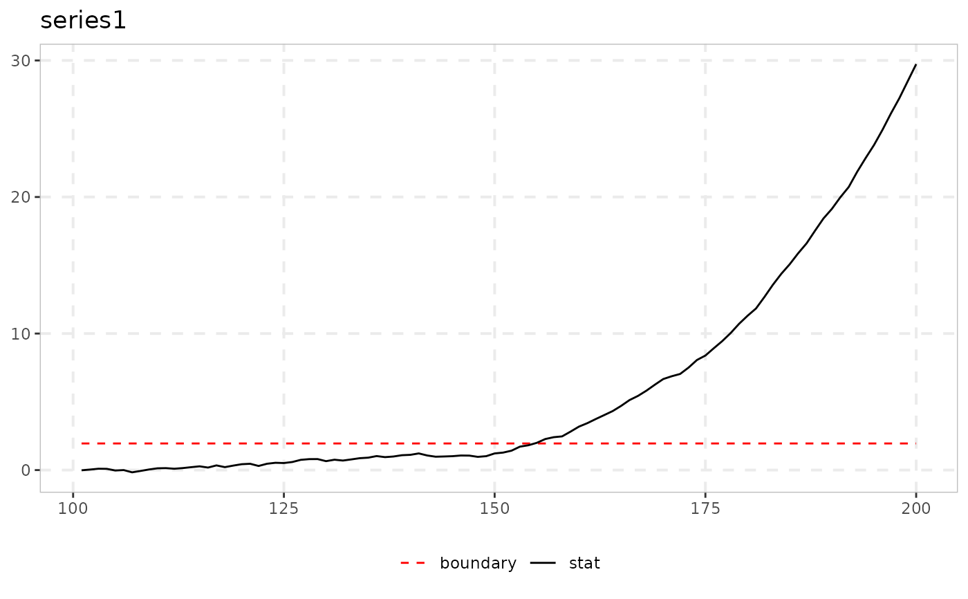
# A martingale training window, explosive from t = 150 to the sample end
y <- sim_psy1(n = 200, te = 150, tf = 200, seed = 7)
res <- monitor_lbi(y, r_star = 100)
print(res) # alarm should fire soon after t = 150
#>
#> ── monitor_lbi (T* = 100 / 200, c_bar = 0, b_alpha = 1.95) ─────────────────────
#>
#> series alarm alarm_date
#> series1 155 155
#>
autoplot(res)
#> Warning: Removed 1 row containing missing values or values outside the scale range
#> (`geom_segment()`).
 # wCUSUM: exponentially up-weight later monitoring observations
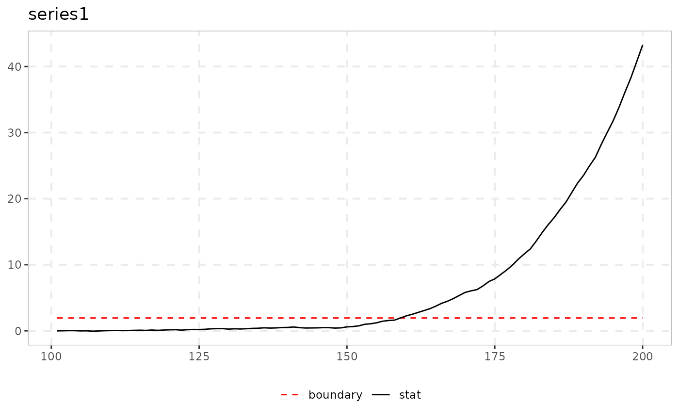
autoplot(monitor_lbi(y, r_star = 100, c_bar = 2))
#> Warning: Removed 1 row containing missing values or values outside the scale range
#> (`geom_segment()`).
# wCUSUM: exponentially up-weight later monitoring observations
autoplot(monitor_lbi(y, r_star = 100, c_bar = 2))
#> Warning: Removed 1 row containing missing values or values outside the scale range
#> (`geom_segment()`).
 # }
# }