QPWY/QPSY Recursive Quantile Monitoring (Wu, Shi & Wu 2025)

monitor_quantile implements the QPWY and QPSY real-time monitoring strategies of Wu, Shi & Wu (2025). They are quantile-regression (QR) analogues of the recursive ADF t-statistics of PWY and PSY, and they test at a chosen conditional quantile tau, in contrast to the single full-sample test in quantile_test. type = "qpwy" uses the expanding window [1, r], which has the shape of badf in radf. type = "qpsy" also takes the supremum over every window start, which has the shape of bsadf.

Usage

monitor_quantile(
  data,
  tau = 0.5,
  minw = NULL,
  nrep = 500L,
  sig_lvl = 95,
  seed = NULL,
  type = c("qpwy", "qpsy"),
  boundary = c("asymptotic", "bootstrap")
)

Arguments

data: A univariate or multivariate numeric time series object, a numeric vector or matrix, or a data.frame. A column may have leading or trailing NA values, which describes an unbalanced panel in which series enter or exit the sample at different times. Those periods are filled with NA in badf and bsadf and excluded from the adf, sadf and gsadf of that series. Interior NA values (a gap in the middle of a series) are not supported. When any series is padded in this way, the panel statistics (bsadf_panel and gsadf_panel) are not available, and the function returns NA for them with a warning.
tau: Quantile to test at, in (0, 1). It is fixed, in contrast to the "optimal" grid search in quantile_test, because eq. 25 of WSW takes tau as a given parameter of the monitoring statistic and does not reselect it at each recursion point.
minw: A positive integer. The minimum window size (default = \((0.01 + 1.8/\sqrt{T})T\), where T denotes the sample size).
nrep: Number of replications for the boundary: Monte Carlo draws of the limit with boundary = "asymptotic", bootstrap resamples with boundary = "bootstrap".
sig_lvl: Significance level, one of 90, 95, 99.
seed: Optional seed for the Monte Carlo draws.
type: "qpwy" (expanding window) or "qpsy" (also the supremum over window starts).
boundary: "asymptotic" (simulated limit, the default) or "bootstrap" (Algorithm 1 of Wu, Shi & Wu 2025).

Value

An object of class monitor_quantile_obj: a list with the statistic path stat, the flat boundary, the estimated delta (reported for both boundaries, used only by the asymptotic one), and alarm and alarm_date (the first breach, NA if there is none).

Details

The point statistic needs genuine QR fits, because there is no closed-form recursive update as there is for OLS. QPWY needs O(T) fits and QPSY needs O(T^2), so QPSY takes seconds for each series at n = 200 and the time grows quadratically.

The boundary is a single flat value and not one value for each r. It is the quantile of the supremum of each null path, constructed like the sadf_cv of radf_mc_cv, which controls the first-crossing false-alarm rate. boundary chooses how the null paths are generated.

With boundary = "asymptotic" (the default) the function simulates the limiting null distribution delta * Q_{r1,r2} + sqrt(1 - delta^2) * Z_{r1,r2} in each call. Here delta is a correlation coefficient estimated from the data (as in quantile_test), Q is the Dickey-Fuller t functional and Z is its counterpart driven by an independent Brownian motion. Both are simulated for every window, so no QR fits are needed and the boundary is cheap.

With boundary = "bootstrap" the function applies Algorithm 1 of Wu, Shi & Wu (2025) to the whole path. It resamples the centred first differences of the series with replacement, cumulates them into a null random walk and recomputes the QPWY or QPSY path on it, nrep times. The boundary is the quantile of the nrep path maxima. It follows the finite-sample distribution of the statistic in the data at hand, so it removes most of the size distortion of the asymptotic boundary described below. Each replicate costs a full statistic path, which is O(T) QR fits for QPWY and O(T^2) for QPSY. The paper also discards the first 100 draws of each resample. We omit this step because the statistic has an intercept, so it does not depend on the level of the series, and the draws are i.i.d., so the retained values already have the same distribution. Set options(exuber.parallel = TRUE) to spread the replicates over workers.

Note

The function simulates the critical value (the boundary) internally in each call, with an unexported helper, quantile_boundary_sim. There is currently no reusable exported cv counterpart for this function. This gap is tracked separately and is not addressed here.

The function returns its own class and not radf_obj, so it does not work with summary(), \link{datestamp} and tidy. It has its own print() and autoplot() methods instead. print() shows the statistic, the boundary and delta. See vignette("naming-and-analysis", package = "exuber") for which functions fit the shared pipeline and which do not.

Caveats

The asymptotic boundary is well sized near the median in finite samples, with a false-alarm rate of 3.5 to 4.0\ innovations, tau = 0.5). Away from the median the small early windows make both statistics oversized, and QPSY badly so even with Gaussian innovations. The false-alarm rate of QPSY is 35\ innovations it is 21\ (n = 100). With \(t_3\) innovations the rate for QPWY is 7.5 to 8.5\ tau = 0.2 and 0.8 and 12.5\ Wu, Shi & Wu advise against extreme quantiles in small samples and use bootstrap critical values for monitoring, which is what boundary = "bootstrap" provides. With it the false-alarm rate was between 4.5 and 6.5\ the cases above (n = 100 for QPWY, n = 60 for QPSY), including QPSY at tau = 0.8 and 0.9. The exception is QPSY with \(t_3\) innovations at tau = 0.9, which stays at 10\ less extreme tau help. For type = "qpsy" with tau away from 0.5 and the asymptotic boundary, the function emits a short pointer as a message (see suppressMessages) and stores it as attr(x, "caveat"). The numbers for both boundaries are in docs/alternative-paradigms.md.

Status

References

Wu, R., Shi, S., & Wu, J. (2025). Quantile analysis for financial bubble detection and surveillance. Journal of Time Series Analysis, 46(5), 908-931.

Examples

# \donttest{
# Heavy-tailed (t3) innovations, explosive from t = 150 to the sample end
y <- sim_psy1(n = 200, te = 150, tf = 200, seed = 7,
  e = sim_innov(199, dist = "t", df = 3))
res <- monitor_quantile(y, tau = 0.5, nrep = 100, seed = 1)
print(res)
#> 
#> ── monitor_quantile (QPWY, n = 200, minw = 27, tau = 0.5, sig_lvl = 95%, asympto
#> 
#>    series  delta  boundary  alarm  alarm_date
#>   series1  0.623     1.934    165         165
#> 
autoplot(res)
#> Warning: Removed 1 row containing missing values or values outside the scale range
#> (`geom_segment()`).


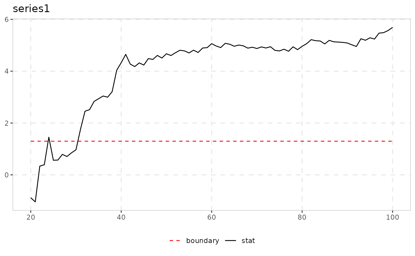# Monitoring an upper quantile is typically more powerful for right-tailed
# bubbles, but see the Caveats section on extreme quantiles
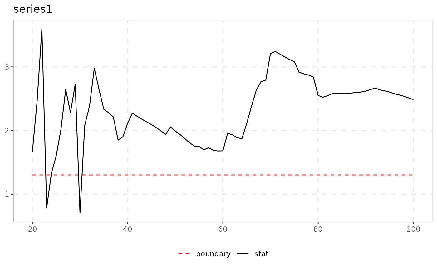
autoplot(monitor_quantile(y, tau = 0.8, nrep = 100, seed = 1))
#> Warning: Removed 1 row containing missing values or values outside the scale range
#> (`geom_segment()`).


# QPSY: supremum over window starts too (O(n^2) QR fits, slower)
monitor_quantile(y[101:200], tau = 0.5, nrep = 100, seed = 1, type = "qpsy")
#> 
#> ── monitor_quantile (QPSY, n = 100, minw = 19, tau = 0.5, sig_lvl = 95%, asympto
#> 
#>    series  delta  boundary  alarm  alarm_date
#>   series1  0.754     2.172     53          53
#> 

# Bootstrap boundary (Algorithm 1 of Wu, Shi & Wu): one full statistic path per
# replicate, so keep nrep small in a first run
monitor_quantile(y, tau = 0.8, nrep = 49, seed = 1, boundary = "bootstrap")
#> 
#> ── monitor_quantile (QPWY, n = 200, minw = 27, tau = 0.8, sig_lvl = 95%, bootstr
#> 
#>    series  delta  boundary  alarm  alarm_date
#>   series1  0.831     1.675    161         161
#> 
# }