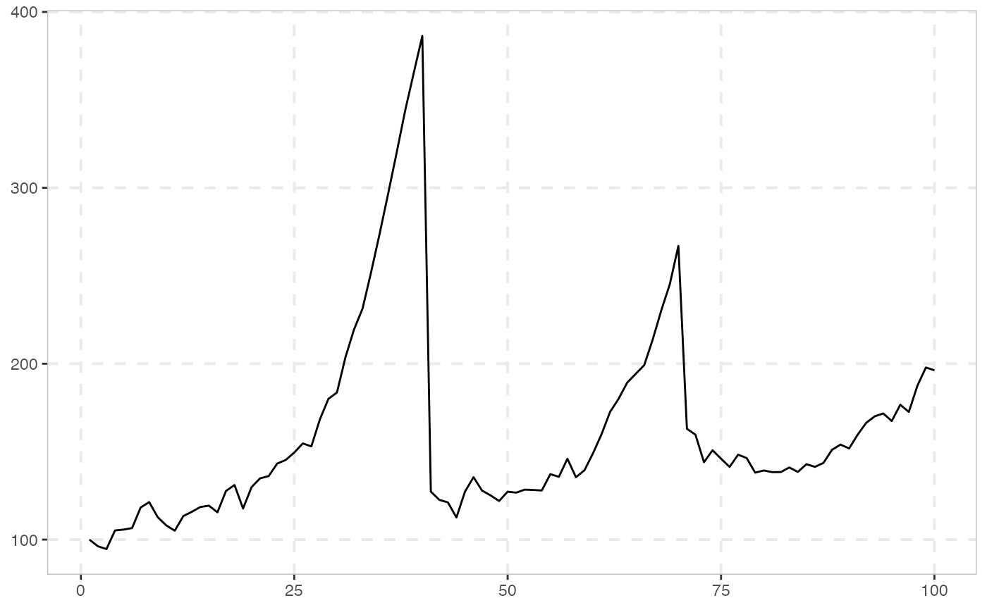
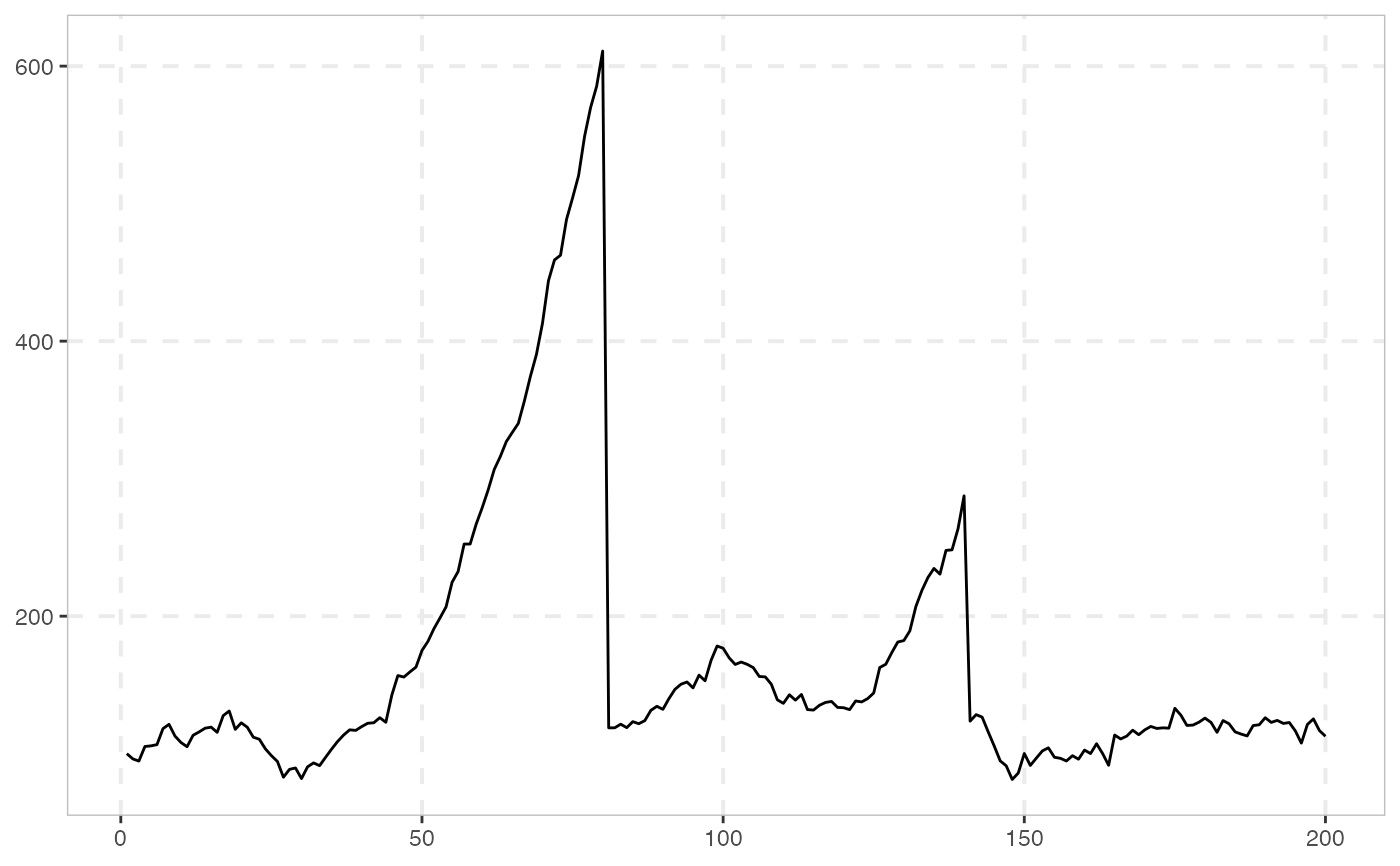
The following data generating process is similar to sim_psy1, with the difference that
there are two episodes of mildly explosive dynamics.
sim_psy2(
  n,
  te1 = 0.2 * n,
  tf1 = 0.2 * n + te1,
  te2 = 0.6 * n,
  tf2 = 0.1 * n + te2,
  c = 1,
  alpha = 0.6,
  sigma = 6.79,
  seed = NULL
)
Arguments
- n
A positive integer specifying the length of the simulated output series.
- te1
A scalar in (0, n) specifying the observation in which the first bubble originates.
- tf1
A scalar in (te1, n) specifying the observation in which the first bubble collapses.
- te2
A scalar in (tf1, n) specifying the observation in which the second bubble originates.
- tf2
A scalar in (te2, n) specifying the observation in which the second bubble collapses.
- c
A positive scalar determining the autoregressive coefficient in the explosive regime.
- alpha
A positive scalar in (0, 1) determining the value of the expansion rate in the autoregressive coefficient.
- sigma
A positive scalar indicating the standard deviation of the innovations.
- seed
An object specifying if and how the random number generator (rng) should be initialized. Either NULL or an integer will be used in a call to
set.seedbefore simulation. If set, the value is saved as "seed" attribute of the returned value. The default, NULL, will not change rng state, and return .Random.seed as the "seed" attribute. Results are different between the parallel and non-parallel option, even if they have the same seed.
Value
A numeric vector of length n.
Details
The two-bubble data generating process is given by (see also sim_psy1):
$$X_t = X_{t-1}1\{t \in N_0\}+ \delta_T X_{t-1}1\{t \in B_1 \cup B_2\} + \left(\sum_{k=\tau_{1f}+1}^t \epsilon_k + X_{\tau_{1f}}\right) 1\{t \in N_1\} $$
$$ + \left(\sum_{l=\tau_{2f}+1}^t \epsilon_l + X_{\tau_{2f}}\right) 1\{t \in N_2\} + \epsilon_t 1\{t \in N_0 \cup B_1 \cup B_2\}$$
where the autoregressive coefficient \(\delta_T\) is:
$$\delta_T = 1 + cT^{-a}$$
with \(c>0\), \(\alpha \in (0,1)\), \(\epsilon \sim iid(0, \sigma^2)\), \(N_0 = [1, \tau_{1e})\), \(B_1 = [\tau_{1e}, \tau_{1f}]\), \(N_1 = (\tau_{1f}, \tau_{2e})\), \(B_2 = [\tau_{2e}, \tau_{2f}]\), \(N_2 = (\tau_{2f}, \tau]\), where \(\tau\) is the last observation of the sample. The observations \(\tau_{1e} = [T r_{1e}]\) and \(\tau_{1f} = [T r_{1f}]\) are the origination and termination dates of the first bubble; \(\tau_{2e} = [T r_{2e}]\) and \(\tau_{2f} = [T r_{2f}]\) are the origination and termination dates of the second bubble. After the collapse of the first bubble, \(X_t\) resumes a martingale path until time \(\tau_{2e}-1\), and a second episode of exuberance begins at \(\tau_{2e}\). Exuberance lasts lasts until \(\tau_{2f}\) at which point the process collapses to a value of \(X_{\tau_{2f}}\). The process then continues on a martingale path until the end of the sample period \(\tau\). The duration of the first bubble is assumed to be longer than that of the second bubble, i.e. \(\tau_{1f}-\tau_{1e}>\tau_{2f}-\tau_{2e}\).
For further details you can refer to Phillips et al., (2015) p. 1055.
References
Phillips, P. C. B., Shi, S., & Yu, J. (2015). Testing for Multiple Bubbles: Historical Episodes of Exuberance and Collapse in the S&P 500. International Economic Review, 5 6(4), 1043-1078.