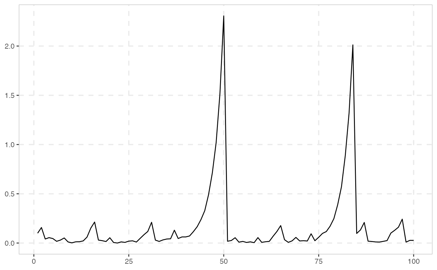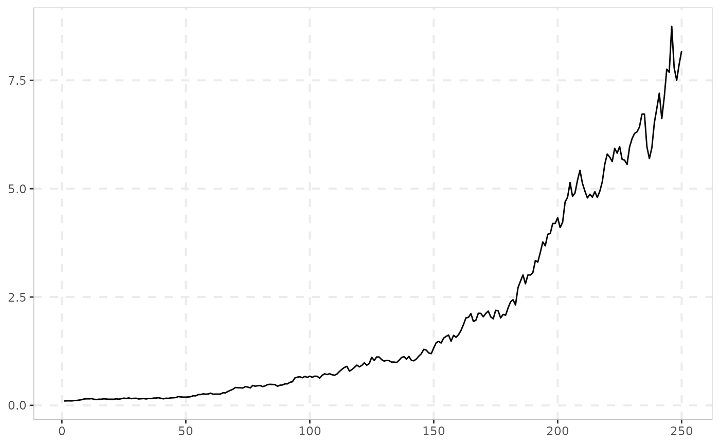
Simulation of a Blanchard (1979) / Rotermann-Wilfling (2018) bubble process

Simulation of a Blanchard (1979) rational bubble process, or (with type = "rotermann_wilfling") Rotermann & Wilfling (2018)'s lognormal-mixture extension of it.

Usage

sim_blan(
  n,
  pi = 0.7,
  sigma = 0.03,
  r = 0.05,
  b0 = 0.1,
  type = c("blanchard", "rotermann_wilfling"),
  delta = 0.984,
  rw_sigma = 0.05,
  seed = NULL
)

Arguments

n: A positive integer specifying the length of the simulated output series.
pi: A positive value in (0, 1) which governs the probability of the bubble continuing to grow.
sigma: A positive scalar indicating the standard deviation of the innovations.
r: A positive scalar that determines the growth rate of the bubble process.
b0: The initial value of the bubble.
type: "blanchard" (default) or "rotermann_wilfling". r is only used by "blanchard"; delta/rw_sigma only by "rotermann_wilfling" (see Details).
delta: A scalar in (0, 1), the Rotermann-Wilfling deflation parameter. Only used for type = "rotermann_wilfling".
rw_sigma: A positive scalar, the standard deviation (on the log scale) of the Rotermann-Wilfling multiplicative lognormal shock. Only used for type = "rotermann_wilfling".
seed: An object specifying if and how the random number generator (rng) should be initialized. Either NULL or an integer will be used in a call to set.seed before simulation. If set, the value is saved as "seed" attribute of the returned value. The default, NULL, will not change rng state, and return .Random.seed as the "seed" attribute. Results are reproducible across the parallel and non-parallel option when the same seed is used.

Value

A numeric vector of length n.

Details

Blanchard's bubble process (type = "blanchard") has two regimes, which occur with probability $\pi$ and $1-\pi$. In the first regime, the bubble grows exponentially, whereas in the second regime, the bubble collapses to a white noise.

With probability $\pi$: $$B_{t+1} = \frac{1+r}{\pi}B_t+\epsilon_{t+1}$$ With probability $1 - \pi$: $$B_{t+1} = \epsilon_{t+1}$$

where r is a positive constant and $\epsilon \sim iid(0, \sigma^2)$.

Rotermann & Wilfling (2018)'s bubble (type = "rotermann_wilfling") replaces the "collapse to white noise" regime with a partial, stochastically evolving deflation, giving periodically recurring, gradually-deflating trajectories instead of an abrupt one-period collapse: $$B_t = \frac{B_{t-1}u_t}{\delta}$$ with probability $\pi$, or $$B_t = \frac{1-\pi\delta}{1-\pi}B_{t-1}u_t$$ with probability $1-\pi$, where $u_t \sim iid\,LN(-rw\_sigma^2/2,\ rw\_sigma^2)$ (so $E[u_t] = 1$). $\delta \in (0, 1)$ ensures the bubble never collapses to exactly zero and can re-inflate.

References

Blanchard, O. J. (1979). Speculative bubbles, crashes and rational expectations. Economics letters, 3(4), 387-389.

Rotermann, B. & Wilfling, B. (2018). "A new stochastic bubble process: Theoretical properties and empirical tests." Applied Economics Letters, 25(15), 1091-1096. As used for Monte Carlo power analysis in Monschang, V. & Wilfling, B. (2021). "Sup-ADF-style bubble-detection methods under test." Empirical Economics, 61, 145-172.

Examples

sim_blan(n = 100, seed = 123) %>%
  autoplot()


sim_blan(n = 250, type = "rotermann_wilfling", delta = 0.984, seed = 123) %>%
  autoplot()