Bubble Contagion Regression (Greenaway-McGrevy & Phillips 2016)

contagion_reg estimates the time-varying contagion coefficient of Greenaway-McGrevy & Phillips (2016). It computes a fixed-window rolling AR(1) coefficient sequence for a "core" series and for a "satellite" series y and relates them with a functional (Nadaraya-Watson kernel) regression at a chosen delay d. The coefficient shows how strongly, and how it varies over time, the local persistence of the core series transmits to y, d periods later.

Usage

contagion_reg(
  y,
  core,
  S = NULL,
  d = 0L,
  h = NULL,
  r_grid = seq(0, 1, length.out = 100)
)

Arguments

y

Satellite (dependent) series, a numeric vector.

core

Core (reference) series, a numeric vector of the same length as y.

S

Fixed rolling-window width for the AR(1) coefficient sequence (default floor(0.33 * length(y)), the choice of the paper).

d

Non-negative integer delay (default 0).

h

Bandwidth for the Nadaraya-Watson regression. The default NULL selects it by leave-one-out cross-validation (eq. 7).

r_grid

Evaluation points for the time-varying coefficient, as fractions of the sample (default seq(0, 1, length.out = 100)).

Value

An object of class contagion_reg_obj: a list with the fixed-window AR(1) coefficient sequences (beta_core and beta_j), the selected or supplied bandwidth (h) and the estimated time-varying contagion coefficient (delta2, aligned with r_grid).

Details

This is a minimal subset of the procedure in the paper. It contains the fixed-window AR(1) coefficient sequence (their eq. 1), the Nadaraya-Watson regression at a single supplied d (eq. 6) and leave-one-out cross-validated bandwidth selection (eq. 7). Their eq. 8, the automatic search over d, is not implemented. If you need a search, call contagion_reg once for each candidate d and compare the fit.

The paper performs no formal inference on the contagion coefficient itself, with no confidence bands and no hypothesis test. As in the paper, this function is a tool for point estimation and visualization and not a test.

Note

The function is not a hypothesis test. It performs no formal inference on the contagion coefficient, with no confidence bands and no significance test, so there is no critical value for it.

The function returns its own class and not radf_obj, so it does not work with summary(), \link{datestamp} and tidy. It has its own print() and autoplot() methods instead. print() shows the coefficient path, because the function performs no formal inference. See vignette("naming-and-analysis", package = "exuber") for which functions fit the shared pipeline and which do not.

Status

References

Greenaway-McGrevy, R., & Phillips, P. C. B. (2016). Hot property in New Zealand: Empirical evidence of housing bubbles in the metropolitan centres. New Zealand Economic Papers, 50(1), 88-113.

See also

cobubble_test for a different, symmetric bivariate bubble relationship that uses a hypothesis test.

Other multivariate: cobubble_test(), radf_common()

Examples

# \donttest{
# A co-explosive pair: the AR coefficient of y follows that of x almost one for one
xy <- sim_coexplosive(n = 100, seed = 123)
res <- contagion_reg(xy$y, xy$x, d = 0L)
print(res)
#> 
#> ── contagion_reg (n = 100, S = 33, d = 0, h = 0.6567) ──────────────────────────
#> 
#> delta_2(r) range: [0.948, 0.965] 
#> 

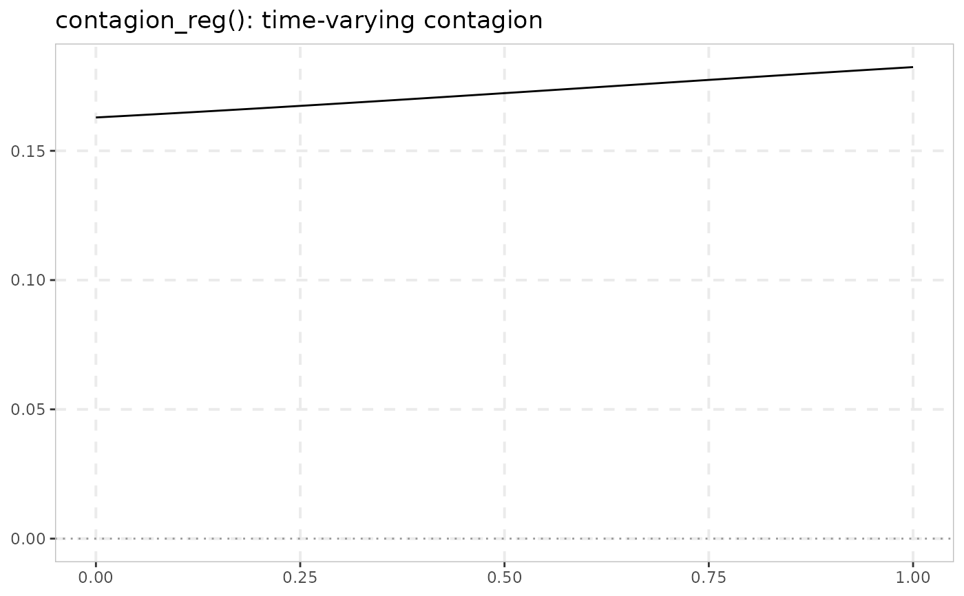
# Plot the estimated time-varying contagion coefficient
autoplot(res)


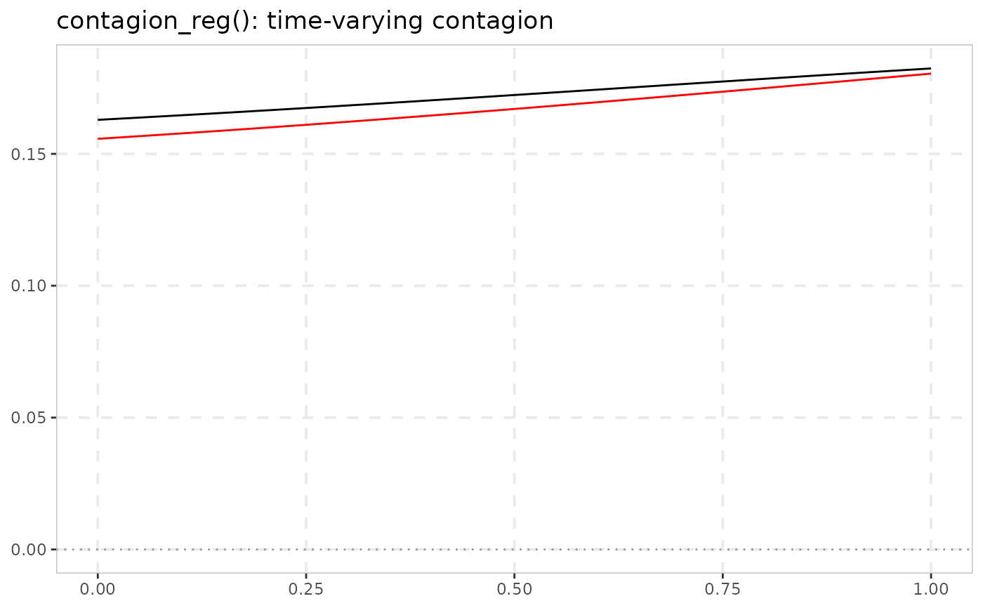
# Compare a one-period lead (d = 1) with the contemporaneous case
res_d1 <- contagion_reg(xy$y, xy$x, d = 1L)
autoplot(res) +
  ggplot2::geom_line(data = data.frame(r = res_d1$r_grid, delta2 = res_d1$delta2),
    ggplot2::aes(r, delta2), color = "red", inherit.aes = FALSE)

# }