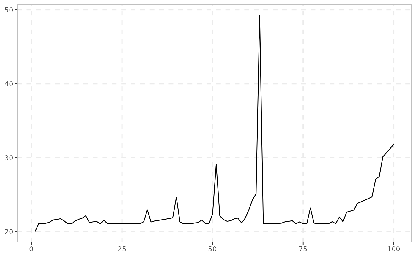
Simulates the stochastic-tree bubble process of Gourieroux & Jasiak (2025). It is
a positive stationary submartingale generated by a binomial tree with
stochastic branching intensity, which makes it a random-coefficient
autoregression, in contrast to the deterministic branches of Cox-Ross-Rubinstein.
The bubble of Blanchard & Watson (1982) (sim_blan) is the special
case of constant intensity.
Usage
sim_tree(
  n,
  a = 0.95,
  eta = 1,
  mu = -1,
  rho = 0.7,
  sigma = 4,
  y0 = eta/(1 - a),
  seed = NULL
)
Arguments
- n
A positive integer specifying the length of the simulated output series.
- a
A scalar in (0, 1) (note: \(1/a > 1\) is the growth rate).
- eta
A positive scalar setting the price floor
eta / (1 - a).- mu, rho, sigma
Parameters of the latent Gaussian AR(1) intensity process (
rhoin (-1, 1),sigma > 0).- y0
Starting value. Defaults to the price floor
eta / (1 - a).- seed
An object specifying if and how the random number generator (rng) should be initialized. It is either NULL or an integer, which is passed to
set.seedbefore the simulation. If you set it, the value is saved as the "seed" attribute of the returned value. The default, NULL, leaves the state of the rng unchanged and returns .Random.seed as the "seed" attribute. Results are reproducible across the parallel and the non-parallel option when you use the same seed.
Details
The stochastic intensity is \(p_t = \Phi(X_t)\), with \(X_t\) a latent stationary Gaussian AR(1): $$X_t = \mu + \rho(X_{t-1}-\mu) + \sigma\sqrt{1-\rho^2}u_t,\quad u_t \sim iid\,N(0,1)$$ Given \(p_t\), draw \(Z_t \sim Bernoulli(p_t)\) and set (the paper's eq. 5-6): $$Y_t = \xi_{1t}Y_{t-1}+\epsilon_t,\quad \xi_{1t}=\frac{1}{a}\frac{Z_t}{p_t},\quad \epsilon_t=\frac{\eta}{1-a}\left(1-\xi_{1t}\right)+\frac{\eta}{a}\frac{1-Z_t}{1-p_t}$$ \(a>1\) controls the growth rate in the active phase of a branch, \(\eta>0\) sets the price floor \(\eta/(1-a)\) (Corollary 1 in the source: \(Y_t \ge \eta/(1-a)\)), \(\rho\) controls the persistence of the bubble-growth phase, and \(\sigma\) controls the frequency of bubbles. The process has no finite mean (Proposition 3 of the source), so occasional very large values are a feature of the model and not a bug.
The default parameters (\(\mu=-1,\eta=1,a=0.95,\sigma=4,\rho=0.7\)) reproduce the illustrative example of the source (Section 2.3, Figure 2).
References
Gourieroux, C. & Jasiak, J. (2025). "A Stochastic Tree for Bubble Asset Modelling and Pricing." JTSA, 46(5), 932-944.